Particles

In this chapter, we will cover the implementation of particles in RAMSES, namely:

• How particles are represented in the code

• How we can we navigate the list of particles in the code

• How particles interact with the grid

1. Particles implementation in RAMSES

1.1 Particle arrays

The core of the particle-related code is stored in the pm folder, where PM stands for “particle-mesh” (i.e., the part of the code responsible for interactions between the particles and the mesh). As for other parts of the code, the majority of the important variables are stored in a commons module. For the particles, the module is pm_commons, found in pm/pm_commons.f90. Additional variables are stored in the corresponding pm_parameters module, located in pm/pm_parameters.f90.

Most quantities related to particles are stored in large global arrays, with in general one variable per array. The size of these arrays is fixed by the maximum number of particles allowed for the run, set by the parameter npartmax defined in the pm_parameters module. We will cover how to set this parameter in the section on the namelist. Just like ngridmax for the grids, the number of particles can either be set directly through npartmax (which sets the maximum number of particles per MPI process), or through the total number of particles across all MPI processes, nparttot. These two are related through nparttot = npartmax*ncpu.

Warning

It is usually more convenient to work with npartmax when developing code, as it is the actual size of the arrays available for each MPI process. However, when running a simulation with a fixed number of particles (e.g., a dark matter-only simulation), nparttot might be more convenient.

The particle masses are stored in the mp variable, which is a one-dimensional array of size npartmax. The positions and velocity are stored in xp and vp, respectively: these are two-dimensional arrays, with size (npartmax, ndim) where ndim is the number of dimensions (usually ndim=3). Similar arrays exist for the birth time, the metallicity, or the AMR level at which the particles are living.

All these arrays are defined in pm/pm_commons.f90:

! Particles related arrays
real(dp),allocatable,dimension(:,:)  ::xp       ! Positions
real(dp),allocatable,dimension(:,:)  ::vp       ! Velocities
real(dp),allocatable,dimension(:)    ::mp       ! Masses
...
real(dp),allocatable,dimension(:)    ::tp       ! Birth epoch
real(dp),allocatable,dimension(:)    ::zp       ! Birth metallicity
...
integer ,allocatable,dimension(:)    ::levelp   ! Current level of particle

1.2 Different types of particles

While RAMSES was originally (Teyssier, 2002) designed to work with only DM particles, the code was quickly extended to star formation, galactic winds, black holes, etc. All these developments have relied, to some extent, on “particles”: for example, stars are modelled as particles representing a stellar population with a unique age and metallicity.

In practice, the choice in RAMSES is that all these “particles” are implemented using the same global arrays: xp for positions, mp for mass, etc. However, this requires some adjustments to identify which particle correspond to what type of thing. For example, some physical models such as supernova explosions only apply to star particles, and we therefore need a simple way to identify which particles corresponds to stars, and which don’t.

Since 2017, RAMSES implements these as particle types (similar, for example, to Gadget/AREPO particle types), stored in the typep array. Contrary to other arrays we have seen so far, typep is not an simple array with real/integer values, instead it is an array of part_t, a derived type that contains two variables, defined at the end of pm/pm_parameters.f90:

• a family variable

• a tag variable

The typep variable is defined in pm/pm_commons.f90:

type(part_t), allocatable, dimension(:) :: typep  ! Particle type array

and the type itself is defined in pm/pm_parameters.f90:

type part_t
   ! We store these two things contiguously in memory
   ! because they are fetched at similar times
   integer(1) :: family
   integer(1) :: tag
end type part_t

The family variable stores what the particle represent:

Family	Value	Physical meaning
FAM_DM	1	DM particle
FAM_STAR	2	Star particle
FAM_CLOUD	3	“Cloud” particle, used for some black-hole implementations
FAM_DEBRIS	4	“Debris” particle, used for some supernovae implementations
FAM_OTHER	5	“Other” type of particle, defined as a catch-all value
FAM_UNDEF	127	Used for “undefined” type, internally

In addition, six other values are used for tracer particles, mirroring values in the table above (e.g., -1 for DM tracers, -2 for star tracers, etc), as well as a FAM_TRACER_GAS=0 value for gas tracer particles.

The particle tags are currently not commonly used, but allow flexibility to have different types of the same kind of particles. For example, one could decide to have Pop III stars and normal Pop II stars implemented at the same time: both would be considered as stars by the code (FAM_STAR family), but still identified independently with their own tag. This can be useful either for post-processing (e.g., “make a map of all Pop III stars”), or even for specific physical models (e.g., Pop III stars could have a different radiative output or stellar evolution model).

In practice, rather than testing directly the typep value of a particle, the best practice is to use the functions defined at the end of the pm_commons module to test whether a particle is of a given type. For example, the is_star function returns True if the particle is a star, and False otherwise. This allows more concise code, as we can write multiple tests in one function. For example, is_tracer returns True if a particle is a tracer particle, irrespective of what kind of tracer.

NB: when implementing new types of particles, make sure to use the right family (if one already exists), use or define the appropriate tag, and (if necessary) add the right tester function.

1.3 Initialising particles

In the code, the global particle arrays are defined in the pm_commons module, but are not allocated there: indeed, npartmax is a runtime parameter, so it cannot be fixed once and for all in the code.

Instead, all the particle-related arrays are allocated when the simulation is initialised, in the init_part routine, defined in pm/init_part.f90. This is done through the following code:

! Allocate particle variables
allocate(xp    (npartmax,ndim))
allocate(vp    (npartmax,ndim))
allocate(mp    (npartmax))

By default, all these arrays are set to 0 prior to proper initialisation. Then, depending on whether the code is starting from initial conditions or re-starting from a previous output, the variables are set to the right values.

When starting from initial conditions, three formats are supported by default: ASCII files, GRAFIC files, and GADGET files. We will not cover the inner details of each of these formats, but the corresponding subroutines (load_ascii, load_grafic, and load_gadget) can all be found in pm/init_part.f90. The easiest to understand is load_ascii, but they all work in similar ways:

1. we read the input file header to deal with units, box size, etc

2. we read all arrays in the input file and count the number of particles

3. (we communicate information across MPI processes)

4. while iterating over particles, we fill the global arrays (xp, vp, mp, etc).

Exercise

Can you explain how the load_ascii and load_grafic subroutines work? For example, can you identify where the positions are read, and where they are set in the xp array?

In the case of a restart, the process is roughly the same, except that each MPI process opens the corresponding file from the last output. For example, if we restart from output 42, the MPI process 37 will open the file output_00042/part_00042.out00037.

Warning

This strategy to initialise the data at restart is part of the reason why RAMSES enforces that the number of MPI processes stays identical when restarting a simulation.

Exercise

Identify where, in init_part.f90, the particle output files are opened.

Solution

Look around if(nrestart>0) then:

call title(nrestart,nchar)
fileloc='output_'//TRIM(nchar)//'/part_'//TRIM(nchar)//'.out'
...
call title(myid,nchar)
fileloc=TRIM(fileloc)//TRIM(nchar)
...
open(unit=ilun,file=fileloc,form='unformatted')

The title function transforms the output number nrestart or the MPI process ID myid to a string padded with five 0.

Once the file is open, we first read a header and then, each array stored in the output will be read. For example, the positions are read as:

! Read position
allocate(xdp(1:npart2))
do idim=1,ndim
   read(ilun)xdp
   xp(1:npart2,idim)=xdp
end do

Let’s explain how these lines work. First, we allocate a temporary array (xdp) with size npart2 corresponding to the number of particles in the file. Then, for each dimension, we read the position from the file to the array xdp, and we fill the position array xp with the array we just read.

Note that we use and re-use several temporary arrays (xdp, isp8, isp, ii1), each corresponding to a data type.

Warning

Careful: if you change the output format for the particles, you will need to change the section of init_part.f90 that deals with restarts.

2. Navigating particle arrays with linked lists

Because of the AMR structure of RAMSES, we need to store particles in a structure that can efficiently be connected to the grid. As the grid evolves with time, this structure also needs to evolve with time. The “natural” solution for this is to use a linked-list for the particles, just like what is done for the grid.

The key idea here is that particles living in the same grid are linked together with a linked-list that is defined per-grid, and we use the grid structure with its own linked list to connect all the particles together.

As this leads to a tree structure, the bulk of the code dealing with the particle list is in the aptly named pm/particle_tree.f90 file.

2.1 Particle linked list structure

In each grid, we have a particle linked list defined using the following variables, defined in pm/pm_commons.f90:

integer ,allocatable,dimension(:)    ::headp    ! Head particle in grid
integer ,allocatable,dimension(:)    ::tailp    ! Tail particle in grid
integer ,allocatable,dimension(:)    ::numbp    ! Number of particles in grid

They are allocated in the init_amr subroutine (in amr/init_amr.f90), if the run parameter flag pic (particle in cell) is set:

if(pic)then
   allocate(headp(1:ngridmax))
   allocate(tailp(1:ngridmax))
   allocate(numbp(1:ngridmax))
   headp=0; tailp=0; numbp=0
endif

Note that if pic is not set, there are no particles, so we don’t have to do any of this.

As required for a linked list, for each particle the next and previous particle in the list is stored. These arrays are defined in pm/pm_commons.f90:

integer ,allocatable,dimension(:)    ::nextp    ! Next particle in list
integer ,allocatable,dimension(:)    ::prevp    ! Previous particle in list

They are allocated in pm/init_part.f90:

allocate(nextp (npartmax))
allocate(prevp (npartmax))

One specificity of particles is that they can move freely through the AMR grid: they can enter and exit cells during a timestep, and (because of the timestepping strategy), they can move to grids that live on different timesteps.

Dealing with this requires careful consideration, and the subroutines dealing with this are found in pm/particle_tree.f90, with the most important one being make_tree_fine. It essentially detaches particles that have moved from their original parent grid, and reattaches them to the grid in which they are now located.

Similarly, when a grid is refined or derefined, special care needs to be taken of the particles: the routines doing this are, respectively, kill_tree_fine and merge_tree_fine.

Finally, when particles move across processor boundaries (see the section on MPI communications), the routine virtual_tree_fine deals with the linked list structure.

2.2 Iterating over particles

The particle and grid linked lists structures are used to iterate over particles.

The following code block represents the usual way of looping over all particles in a given MPI process:

do icpu=1,ncpu
! Loop over cpus
   igrid=headl(icpu,ilevel)
   ! Loop over grids
   do jgrid=1,numbl(icpu,ilevel)
      npart1=numbp(igrid)  ! Number of particles in the grid
      if(npart1>0)then
         ipart=headp(igrid)
         ! Loop over particles
         do jpart=1,npart1
            ! Save next particle   <--- Very important !!!
            next_part=nextp(ipart)

            !----
            ! Do something with particle ipart
            !----

            ipart=next_part  ! Go to next particle
         end do
      endif
      igrid=next(igrid)   ! Go to next grid
   end do
end do

Let’s unravel this and start from the igrid = headl(icpu, ilevel) line. This initialises the variable igrid to the index of the first element of the list of grids at the current level ilevel.

Then, the section

do jgrid=1, numbl(icpu, ilevel)
    npart1=numbp(igrid)
    ...
    igrid=next(igrid)
end do

loops over all grids at the current level. The variable npart1=numbp(igrid) stores the number of particles that exist in grid indexed by igrid. Note here that when we first enter the loop, igrid is defined from the headl access, but at the end of the loop, we go to the next grid in the list, determined by next(igrid).

If there is at least one particle in the grid (i.e., if npart1>0), we can loop over the particles in the grid with the particle linked-list:

ipart=headp(igrid)
do jpart=1,npart1
    next_part=nextp(ipart)
    ...
    ipart=next_part
end do

This is done in many places in the code, and looking for the Very important !!! comment is likely to return many of these places. You can guess how people usually go about writing this loop.

2.3 Adding and deleting new particles

Multiple routines in RAMSES need to create or destroy particles. Once again, the most typical example is the star formation routine: when new stars are formed, we need to “spawn” new particles and update the linked lists accordingly. Conversely, it can happen that particles are destroyed (for example, the “cloud particles” surrounding black holes when two black holes merge).

This is handled by routines found in pm/add_list.f90 and pm/remove_list.f90. Let’s quickly review how they work together.

When spawning new particles, we need to insert them somewhere in the particle linked list. This is done relatively easily thanks to the linked list structure: we just need to add the particle index after the current last particle in the nextp array. This is essentially what the add_list subroutine does in pm/add_list.f90:

nextp(tailp(ind_grid(j))) = ind_part(j)

Here, tailp(ind_grid(j)) indicates the tail of the particle linked list in the grid ind_grid(j), and we define the nextp particle as the one with index ind_part(j).

To make sure that there is enough space in the particle arrays, we need to use the remove_free subroutine of pm/remove_list.f90, which essentially reserves a block of the particle arrays for the new particles.

As a result, the correct way to update the linked lists when adding new particles is always to first call remove_free, then add the particles with add_list. This is for example done in the star formation routine in pm/star_formation.f90:

! Update linked list for stars
call remove_free(ind_part,nnew)
call add_list(ind_part,ind_grid_new,ok_new,nnew)

3. Cloud-in-Cell scheme

Particles interact with the rest of the simulation in essentially two ways: either through direct exchange of mass, energy, momentum, radiation (…) with the grid, or through their gravitational influence. The former will be discussed in the section on subgrid modelling, and we will now focus on the way particles interact with gravity.

CIC is a general mapping between grids and particles: it can be used beyond gravity (e.g., for sink particles accretion). As discussed in the section on subgrid modelling, other assignment schemes are used for feedback, for example.

3.1 Overview

As already discussed in the general review of the code, (massive) particles act as a source term for gravity: they contribute to the density field \(\rho\). This field is represented in the code by the rho array, which is defined for each cell. In order for particles to contribute to the density field, we need a method to distribute their mass on the grid.

RAMSES does this through the cloud-in-cell scheme, or CIC. The idea is to distribute the mass of each particle in a cloud with cubic shape (in 3D): unless the particle is perfectly at the centre of a cell, its cloud will overlap with other cells, and the mass of the particle will be spread over those cells depending on the volume fraction of the overlapping region.

In more details: a particle that “lives” at a level ilevel will be represented as a cube with side length \(\Delta x = L/2^{\texttt{ilevel}}\), and its volume will therefore be \(\Delta x^{\texttt{ndim}}\), usually \(\Delta x^3\). We can show that the cloud will overlap with \(2^{\texttt{ndim}}\) grid cells. In order to compute the contribution of a particle to each of the overlapping cells, we need:

• the indices of the cells with which the particle overlaps

• the overlapping sub-volume of the particle cloud with these cells.

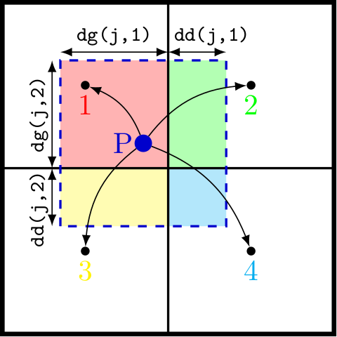
In practice, the second part is done before the first: the sub-volumes are calculated as rectangular cuboids, using the distances to the cell boundaries dd and dg (respectively for distance droite and distance gauche).

3.2 Walking through cic_amr

To better understand how the CIC scheme is applied, let’s look at the cic_amr routine that can be found in the pm/rho_fine.f90 file.

After some book-keeping, we recover the neighbouring father cells with

call get3cubefather(ind_cell,nbors_father_cells,ng,ilevel)

This will be needed to get the grid index of all the neighbours.

We then rescale all the positions at the current level to get the position of the 3×3×3 neighbour grids (in 3D), rescaled to be between 0 and 6 in each dimension.

! Rescale particle position at level ilevel
do idim=1,ndim
   do j=1,np
      x(j,idim)=xp(ind_part(j),idim)/scale+skip_loc(idim)
      x(j,idim)=x(j,idim)-x0(ind_grid_part(j),idim)
      x(j,idim)=x(j,idim)/dx
   end do
end do

This is then the time to get the particle properties that we may want to dump on the grid, for example the mass of non-tracer particles. This is done by reading the particle mass mp in the cic_amr routine, but we could do the same thing for other extensive quantities (e.g., metal mass).

After some extra checks, we then compute dd and dg along each dimension. The volume of each of the sub-volumes is computed from the values of dg and dd. For example, in two dimensions:

#if NDIM==2
  do j=1,np
     vol(j,1)=dg(j,1)*dg(j,2)
     vol(j,2)=dd(j,1)*dg(j,2)
     vol(j,3)=dg(j,1)*dd(j,2)
     vol(j,4)=dd(j,1)*dd(j,2)
  end do
#endif

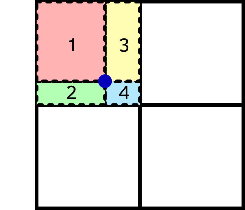
Particle j will have a fraction of its cloud volume in cell #1 given by dg(j,1)*dg(j,2), the fraction in cell #2 given by dd(j,1)*dg(j,2), and so on. All these are stored in the array vol(:,:), where the first dimension corresponds to the particle, and the second to the sub-volume.

Once this is all computed, we need to assign these sub-volumes to the relevant cells.

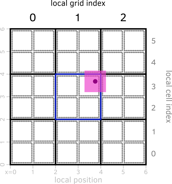
First, we need to identify the local index of the parent grid. During the dd and dg computation, we get the index of the left and right boundaries in ig and id, respectively. As the parent grid lives on level ilevel-1, the corresponding local) grid indices (igg and igd, for index grid gauche and index grid droite) will be halved:

do idim=1,ndim
   do j=1,np
      igg(j,idim)=ig(j,idim)/2
      igd(j,idim)=id(j,idim)/2
   end do
end do

On the figure above, this corresponds to computing the local grid index from the local position.

From there, we compute an index kg for each of the 8 sub-volumes, which is used to determine the global grid index igrid of that parent grid:

do ind=1,twotondim
   do j=1,np
      igrid(j,ind)=son(nbors_father_cells(ind_grid_part(j),kg(j,ind)))
   end do
end do

We then need to determine which of the 8 cells belonging to the parent grid is relevant, i.e., which is the local ind (as defined in the section on AMR structure). This is done again by index arithmetics, depending on the values of ig, id, igg, and igd, and yields the array icell(:,:) where the first dimension corresponds to the particle on which we are working, and the second to the 8 sub-volumes.

We finally can compute the global cell index as

! Compute parent cell adress
do ind=1,twotondim
   do j=1,np
      indp(j,ind)=ncoarse+(icell(j,ind)-1)*ngridmax+igrid(j,ind)
   end do
end do

Once all of this is done, we can loop over the particles to do something with the CIC scheme. For example, in cic_amr, we compute the contribution of the particles to the density array rho: we first define the “mass fraction” vol2:

do j=1,np
   ok(j)=(igrid(j,ind)>0).and.is_not_tracer(fam(j))
   vol2(j)=mmm(j)*vol(j,ind)/vol_loc
end do

and then increment rho with it:

do j=1,np
   if(ok(j))then
      rho(indp(j,ind))=rho(indp(j,ind))+vol2(j)
   end if
end do

3.3 Details of the CIC density calculation

If we look more carefully at the main loop where the density field is computed, we can note several things.

if(cic_levelmax==0.or.ilevel<=cic_levelmax)then
   do j=1,np
      if(ok(j))then
         rho(indp(j,ind))=rho(indp(j,ind))+vol2(j)
      end if
   end do
else if(ilevel>cic_levelmax)then
   do j=1,np
      ! check for non-DM (and non-tracer)
      if ( ok(j) .and. is_not_DM(fam(j)) ) then
         rho(indp(j,ind))=rho(indp(j,ind))+vol2(j)
      end if
   end do
endif

if(ilevel==cic_levelmax)then
   do j=1,np
      ! check for DM
      if ( ok(j) .and. is_DM(fam(j)) ) then
         rho_top(indp(j,ind))=rho_top(indp(j,ind))+vol2(j)
      end if
   end do
endif

First of all, for DM particles, CIC assignment is only done if the level is below cic_levelmax. Otherwise, a different array, rho_top is updated. This is a way of dealing with the fact that DM particles are usually much more massive than the baryons in the simulation. In practice, this “smooths” the DM particles to the level cic_levelmax, which is a free namelist parameter.

Warning

A good way of choosing cic_levelmax is to run a DM-only simulation, and see what is the maximum level of refinement that is reached. This will be the natural smoothing level for the DM particles, and avoids dumping all the DM particle mass in a small cell (whose size is determined by its baryonic content rather than DM content).

This is note done for non-DM particles: indeed, they are expected to “live” at the finest grid level.

Second, we can also note that CIC is used in several places.

• cic_amr called from rho_from_current_level, itself called in rho_fine, which calculates the density field of the particles.

• cic_cell called from cic_from_multipole which represents the gas cells as pseudo-particles to calculate the gas density field (used as input for the gravity calculation) in the same way as the particles. This has some advantages.

• cic_only called from rho_only_level in the clumpfinder, to calculate the density field on which to perform the clump finding.

While all these routines are pretty similar, this leads to a lot of code duplication, which can sometimes be hard to maintain. There is work being done on this, but it takes time.

Also, RAMSES has an alternative to the CIC scheme that is in principle more accurate: the TSC scheme, for triangular-shaped cloud. This is a smoother, more expensive, assignment scheme.

Exercise

Go through the code for the TSC scheme. What is different about it?

3.4 Inverse CIC: grid affecting the particles

As we have seen in the gravity section, once the Poisson equation has been solved, we need to update the particle positions and velocities. As the acceleration (from the gravitational field) is only known at the grid position, we need to interpolate it at the particle positions.

This is done using the same type of CIC scheme as for the density calculation, except that instead of changing a quantity on the grid, we read the updated force at the particle location. Just like previously, we need:

• the identity of each neighbouring cell

• the fraction of the particle cloud in each neighbouring cell

• the contribution of each of these cell to the acceleration

Note that special care must be taken when the particle overlaps with cells that are at a different refinement level.

As an exercise, you can go through the sync routine called by synchro_fine in pm/synchro_fine.f90 and move1 called by move_fine in pm/move_fine.f90 to go through the logic.