Godunov solver#
1. Solving hydro with the Finite Volume Method (FVM)#
Several numerical methods exist to solve the hydrodynamic equations on a grid. RAMSES uses a finite volume method, more specifically an explicit second-order predictor-corrector Godunov scheme (see further), to integrate this conservative system of equations. This subset of methods is particularly well-suited for solving hyperbolic systems of conservation laws like the Euler equations. The method ensures conservation of mass, momentum, and energy across cell boundaries by construction.
In finite volume methods, the computational domain is discretized into control volumes \(V_i\) called cells. Remark that when using AMR, these volumes can have different sizes. Writing the system equation in integral form results in
\(\frac{d}{dt} \int_{V_i} \mathbb{U} \, dV + \int_{\partial V_i} \mathbb{F} \cdot \hat{n} dS, dA = \int_{V_i} \mathbb{S} \, dV\)
When defining the cell-averaged conserved quantities as
\(\mathbb{U}_i(t) = \frac{1}{|V_i|} \int_{V_i} \mathbb{U}(\mathbf{x}, t) \, dV ,\)
and the numerical flux through face \(f\) as \(\mathbb{F}_f\), the semi-discrete update of the conservative variables becomes:
\(\frac{d \mathbb{U}_i}{dt} = -\frac{1}{|V_i|} \sum_{f \in \text{faces}} \mathbb{F}_f A_f + \mathbb{S}_i\)
with \(A_f\) the area of face \(f\) and \(\mathbb{S}_i\) the cell-averaged source term.
Numerical fluxes \(\mathbb{F}_f\) are obtained by solving Riemann problems at each interface between cells (see further), using the states on the left \(\mathbb{U}_L\) and right \(\mathbb{U}_R\) of the interface. For this, the interface states themselves first have to be interpolated from the cell-centered values. To compute the fluxes RAMSES used the MUSCL-Hancock scheme, which is a second-order Godunov method (more on this further).
Discretizing further, the conservative variable update becomes (in 1D):
\(\mathbb{U}_i^{n+1} = \mathbb{U}_i^{n} - \frac{\Delta t}{\Delta x} (\mathbb{F}_{i+1/2} - \mathbb{F}_{i-1/2}) + \Delta t \, \mathbb{S}_i\)
where \(\mathbb{F}_{i\pm1/2}\) are the fluxes going through opposing faces of the cell.
In the code, the entry point for hydro solver is godunov_fine. This
routine uses the standard RAMSES structure to gather nvector cells
to be send of to the core calculation routine godfine1.
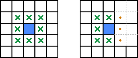
Inside godfine1, the first step is to gather a stencil of 6 x 6 x 6
cells (in 3D) neighboring cells (this is needed to have second order
accurary in the slope calculation, see later). If there is AMR, the
neighboring cells may not be on the same refinement level and an
interpolation is performed. In that case, the coarse level is virtually
refined at the fine level, and the hydro variables are interpolated
(done by the routine interpol_fine).
Then, the subroutine unsplit is called, which calculates the fluxes.
The name comes from the implementation being ‘unsplit’, meaning that the
fluxes are computed simultaniously for all spatial directions (see
further). The fluxes are always computed at the left side of the cell.
Finally, at the end of godfine1, unew is updated using the
fluxes from all directions (unsplit method).
How source terms are treated will be discussed further.
2. Unsplit MUSCL-Hancock scheme for computing the fluxes#
By default, RAMSES uses the MUSCL-Hancock scheme for computing the numerical fluxes across cell faces. This is a predictor-corrector extension of Godunov’s method that allows for second-order accuracy by using
piecewise linear reconstruction of the cell states, in contrast to Godunov’s original piecewise constant
a half step prediction for time evolution.
The scheme is extended to multiple dimension in an unsplit fashion,
which is why the corresponding entry subroutine is named unsplit.
This means that the fluxes in all directions are computed at the same
time, that is in one timestep. Transverse corrections are included. This
approach avoids splitting errors, better preserves symmetry and is
overall more accurate for multi-dimensional simulations.
The steps for obtaining the flux are as follows.
Convert conservative cell-centered variables to primitive variables (
ctoprim)Calculate the limited slopes (TVD) for the primitive variables that will be used to reconstruct the state at the cell edges and evaluate space derivative for the time evolution below (MUSCL part,
uslope)Evolve (or
trace) the cell centered states forward in time for half a time step and then project on cell faces (Hancock part).Solve the Riemann problem at each interface using predicted left/right states to obtain the fluxes \(F_{i+1/2}\)
cmpflxm(“compute flux minus”, because only the left flux is calculated)
These fluxes are then used to update the conserved variables. Below, we go into each step in more detail. You can visit the following page for a more complete description of the MUSCL-Hancock scheme: https://ammar-hakim.org/sj/hancock-muscl.html
Switch to primitive variables#
First, the conservative variables are converted into their primitive
form. This is done by the subroutine ctoprim, which has as input the
cell-centered conservative variables \(\mathbb{U}\) and as output
the corresponding primitive variables \(\mathbb{Q}\).
While not strictly required, it has become standard practice to use primitive variables for higher-order Godunov schemes like the MUSCL-Hancock scheme. This choice improves both accuracy and stability of the method. Primitive variables tend to vary more smoothly, especially across contact discontinuities and shocks, making them better suited for linear reconstruction and slope limiting. Reconstructing in conserved variables can introduce spurious oscillations or unphysical states such as negative densities or pressures. By switching to primitive variables during reconstruction and time prediction, the scheme maintains physical realism while achieving second-order accuracy.
A subtlety arises when gravity is included in the simulation. In that case, half a gravity predictor step is applied to the velocity in this routine. See more further.
Compute the slopes#
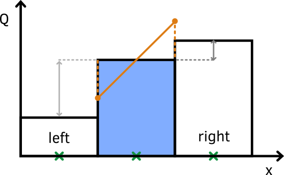
In the MUSCL-Hancock scheme, the goal of the reconstruction step is to approximate the solution inside each cell using a linear profile, instead of a constant value. Given the cell-averaged primitive variables \(Q_i\), the slope \(\Delta Q_i\) is computed using the cell-centered values of the neighboring cells. A slope limiter is applied to control oscillations near discontinuities:
\(\Delta Q_i = \text{Limiter}(Q_{i+1}-Q_i, Q_i - Q_{i-1})\)
For example, the average slope without limiting would be simply
\(\Delta Q_i = \frac{(Q_{i+1} - Q_i) + (Q_i - Q_{i-1})}{2}\),
which can introduce new extrema in the reconstructed field. This configuration is prone to oscillations. Total variation diminishing (TVD) limiters prevent the apparition of these spurious oscillations.
In RAMSES, calculating the limited slope is done by the subroutine
uslope. Several slope limiters are implemented (minmod, monotonized
centered, etc…).
Predictor step: evolution of cell boundary values for half a time step#
The predictor step advances these states forward by half a timestep to account for their local evolution (Source term part) and reconstruct the state at the left and right interface of the cell. This increases temporal accuracy to second order.
First, the cell centered primitive variables are advanced for hal a timestep. The evolution is governed by the Euler equations, linearized around the reconstructed primitive states. In practice, this is done by applying the method of lines to estimate the time derivative and then updating the interface states. In 1D
\(\rho^{n+1/2}_i=\rho^n_i - (u^n_i\Delta_x \rho^n_i+\rho^n_i\Delta_x u^n_i)\Delta t/\Delta x\)
\(u^{n+1/2}_i=u^n_i - (u^n_i\Delta_x u^n_i+\Delta_x P^n_i/\rho^n_i)\Delta t/\Delta x\)
In the case of multiple dimensions, transverse corrections are applied, accounting for the coupling between spatial directions. These are cross-derivative terms that arise when wave propagation in one direction is affected by gradients in perpendicular directions, which is crucial for preserving accuracy and symmetry in 2D and 3D flows.
In 2D
\(\rho^{n+1/2}_i=\rho^n_i - (u^n_i\Delta_x \rho^n_i+\rho^n_i\Delta_x u^n_i)\Delta t/\Delta x - (u^n_i\Delta_y \rho^n_i+\rho^n_i\Delta_y u^n_i)\Delta t/\Delta y\)
\(u^{n+1/2}_i=u^n_i - (u^n_i\Delta_x u^n_i+\Delta_x P^n_i/\rho^n_i)\Delta t/\Delta x - (v^n_i\Delta_y u^n_i)\Delta t/\Delta y\)
\(v^{n+1/2}_i=v^n_i - (u^n_i\Delta_x v^n_i)\Delta t/\Delta x - (v^n_i\Delta_y v^n_i +\Delta_y P^n_i/\rho^n_i)\Delta t/\Delta y\)
Then, we define left and right interface states at the boundaries of each cell:
\(Q_i^m = Q_i^{n+1/2} - \frac{1}{2} \Delta Q_i\\ Q_i^p = Q_i^{n+1/2} + \frac{1}{2} \Delta Q_i\)
These reconstructed values represent the linearly extrapolated states at each interface, from within cell ii. This reconstruction is applied in each spatial direction independently.
The predictor step is perfomed in the subroutine trace
Solving the Riemann problem to obtain the fluxes through cell interfaces#
The last step is to compute the flux through the cell faces given the states to the left and right of the interface. This is a Riemann problem, i.e. a discontinuity with a value on the left and another value on the right, which can be solved numerically using Riemann solvers. RAMSES users have the choice between several different Riemann solvers. For more info on Riemann solvers, see elsewhere.
In the code, the subroutine cmpflxm is called for each spatial
direction. Inside cmpflxm, the requested Riemann solver is called.
The output array flux is then updated with the 1D flux for the
requested spatial direction.
If AMR is active, the coarse level is updated during the fine level update at fine-to-coarse boundary.
Exercise
Find in the code where the coarse level is virtually refined. Does it imply some interpolation?
Find in the code where the coarse level update is done? What does it imply for conservative variable evolution? What about coarse-to-fine boundary?
Solution
in ‘umuscl.f90’. Quantities are conserved. The coarse-to-fine boundary is never considered, the flux being set to zero.