Getting started#
In this chapter, we will explain step by step how to get the RAMSES package and install it, then how to perform a simple test to check the installation.
Obtaining the package#
The package can be downloaded from the GitHub repository using git:
$ git clone https://github.com/ramses-organisation/ramses
This will create a new repository called ramses/
In this directory, you will see:
$ ls -F
README		bin/		mhd/		patch/		rt/
amr/		doc/		namelist/	pm/		utils/
aton/		hydro/		pario/		poisson/
Each directory contains a set of files with a given common purpose.
For example, amr/ contains all Fortran 90 routines dealing with the
AMR grid management and MPI communications, while hydro/ obviously
contains all Fortran 90 routines dealing with hydrodynamics. The
first directory you are interested in is the bin/ directory, in which
the code will be compiled.
Compiling the code#
You need to go first to the bin/directory:
$ cd ramses/bin
$ ls -F
Makefile	Makefile.rt
We will use the first Makefile to compile the code. The first thing
to do is to edit the Makefile and modify the two variables F90 and
FFLAGS. Several examples corresponding to different Fortran
compilers are given. The default values are:
F90 = gfortran -O3 -frecord-marker=4 -fbacktrace -ffree-line-length-none
FFLAGS = -x f95-cpp-input -DWITHOUTMPI $(DEFINES)
The first variable is obviously the command used to invoke the Fortran
compiler. In this case, this is the GNU Fortran compiler. The
second variable contains Fortran compilation flags and preprocessor
directives. The first directive, -DWITHOUTMPI, switches off all MPI
routines. On the other hand, if you don’t use this directive, the
code must be linked to the MPI library. We will discuss this point
later.
Other preprocessor directives are defined in variable DEFINES in the
Makefile:
# Compilation time parameters
NVECTOR = 64
NDIM = 3
NPRE = 8
NVAR = 8
SOLVER = hydro
PATCH =
EXEC = ramses
DEFINES = -DNVECTOR=$(NVECTOR) -DNDIM=$(NDIM) -DNPRE=$(NPRE) -DNVAR=$(NVAR) -DSOLVER$(SOLVER)
These additional directives are called Compilation Time
Parameters. They should be defined in the Makefile and the code must
be recompiled entirely using:
$ make clean
$ make
We list now the definitions of these parameters.
NVECTOR=64
: This parameter is used to set the vector size for
computation-intensive operations. It must be determined
experimentally on each new hardware.
NPRE=4
: This parameter sets the precision of the floating point operations.
NPRE=4stands for single precision arithmetics, while NPRE=8 is
for double precision.
NENER=0
: This parameter sets the number of energy variables used in the hydro or mhd solver.
NDIM=3
: This parameter sets the dimensionality of the problem.
The value NDIM=1is for 1D, plan-parallel flows. NDIM=2 and
NDIM=3 are resp. for 2D and 3D flows.
SOLVER=hydro
: This parameter selects the type of hyperbolic solver used.
Possible values are: hydro for the adiabatic Euler equations,
mhd, the Constrained Transport scheme for the ideal MHD equations.
and rhd for relativistic hydro.
NVAR=8
: This parameters defines the number of variables in the hyperbolic solver.
For SOLVER=hydro, NVAR>=NDIM+2.
For SOLVER=mhd, NVAR>=8 and for SOLVER=rhd, one has NVAR>=5.
Our goal is now to compile the code for a simple one-dimensional problem.
You need to modify the Makefile so that:
NDIM=1
SOLVER=hydro
NVAR=3
Then type:
$ make
If everything goes well, all source files will be compiled and
linked into an executable called ramses1d.
Additional compilation preprocessor flags#
-DTSC
: This parameter sets the triangular shape cloud approximation; only works with NDIM=3
-DOUTPUT_PARTICLE_POTENTIAL
: This parameter forces the code to output particle potentials at snapshots
-DQUADHILBERT
: This parameter sets longer Hilbert curve necessary if levelmax>19
-DLONGINT
: This parameter switches to long ints (necessary when one has lots of particles)
-DNOSYSTEM
: This parameter handles operating system commands
Executing the test case#
To test the compilation, you need to execute a simple test case. Go up one level and type the following command:
$ cd trunk/ramses
$ bin/ramses1d namelist/tube1d.nml
The first part of the command is the executable we have just compiled.
The second part, the only command line argument, is an input file
containing the run time parameters. Several examples of such parameter
files are stored in the namelist/ directory. The namelist file we
have just used tube1d.nml is the Sod test, a simple shock tube simulation
in 1D. For comparison, we now show the last 14 lines of the standard output:
 Mesh structure
 Level  1 has          1 grids (       1,       1,       1,)
 Level  2 has          2 grids (       2,       2,       2,)
 Level  3 has          4 grids (       4,       4,       4,)
 Level  4 has          8 grids (       8,       8,       8,)
 Level  5 has         16 grids (      16,      16,      16,)
 Level  6 has         27 grids (      27,      27,      27,)
 Level  7 has         37 grids (      37,      37,      37,)
 Level  8 has         17 grids (      17,      17,      17,)
 Level  9 has         16 grids (      16,      16,      16,)
 Level 10 has         13 grids (      13,      13,      13,)
 Main step=    43 mcons=-1.97E-16 econs= 1.61E-16 epot= 0.00E+00 ekin= 1.38E+00
 Fine step=   688 t= 2.45047E-01 dt= 3.561E-04 a= 1.000E+00 mem= 7.6%
 Run completed
If your execution looks similar, it means your installation was successfull. Users are encouraged to redirect the standard output into a log file. This log file contains all simulation control variables, as well as output variables, but for 1D simulations only.
$ bin/ramses1d namelist/tube1d.nml > tube.log
Reading the log file#
We will now briefly describe the structure and the nature of the
information available in the log file. We will use as example the file
tube.log we have just created. It should contain, starting from the top:
 _/_/_/       _/_/     _/    _/    _/_/_/   _/_/_/_/    _/_/_/
 _/    _/    _/  _/    _/_/_/_/   _/    _/  _/         _/    _/
 _/    _/   _/    _/   _/ _/ _/   _/        _/         _/
 _/_/_/     _/_/_/_/   _/    _/     _/_/    _/_/_/       _/_/
 _/    _/   _/    _/   _/    _/         _/  _/               _/
 _/    _/   _/    _/   _/    _/   _/    _/  _/         _/    _/
 _/    _/   _/    _/   _/    _/    _/_/_/   _/_/_/_/    _/_/_/
                         Version 3.0
        written by Romain Teyssier (CEA/DSM/IRFU/SAP)
                      (c) CEA 1999-2007

 Working with nproc =    1 for ndim = 1
 Using the hydro solver with nvar =  3

 Building initial AMR grid
 Initial mesh structure
 Level  1 has          1 grids (       1,       1,       1,)
 Level  2 has          2 grids (       2,       2,       2,)
 Level  3 has          4 grids (       4,       4,       4,)
 Level  4 has          8 grids (       8,       8,       8,)
 Level  5 has          8 grids (       8,       8,       8,)
 Level  6 has          8 grids (       8,       8,       8,)
 Level  7 has          8 grids (       8,       8,       8,)
 Level  8 has          8 grids (       8,       8,       8,)
 Level  9 has          6 grids (       6,       6,       6,)
 Level 10 has          4 grids (       4,       4,       4,)
 Starting time integration
 Output    58 cells
 ================================================
 lev      x           d          u          P
  4  3.12500E-02  1.000E+00  0.000E+00  1.000E+00
  4  9.37500E-02  1.000E+00  0.000E+00  1.000E+00
...
  4  9.06250E-01  1.250E-01  0.000E+00  1.000E-01
  4  9.68750E-01  1.250E-01  0.000E+00  1.000E-01
 ================================================
 Fine step=     0 t= 0.00000E+00 dt= 6.603E-04 a= 1.000E+00 mem= 3.2%
 Fine step=     1 t= 6.60250E-04 dt= 4.420E-04 a= 1.000E+00 mem= 3.2%
After the code banner and copyrights, the first line indicates that you are currently using 1 processor and 1 space dimension for this run. The second line confirms the solver used and the number of variables defined for this run. The code then reports that it is building the initial AMR grid. The next lines give the resulting mesh structure.
The first level of refinement in ramses covers the whole computational
domain with 2 (resp. 4 and 8) cells in 1 (resp. 2 and 3) space dimension.
The grid is then entirely refined up to levelmin, which in this case is
defined in the parameter file to be levelmin=3. This defines the
coarse grid. The grid is then adaptively refined up to levelmax, which
in this case levelmax=10. Each line in the log file indicates the
number of octs (or grids) at each level of refinement. The maximum number
of grids in each level level is equal to 2**(level-1) for NDIM=1,
to 4**(level-1) for NDIM=2 and to 8**(level-1) for NDIM=3.
The numbers inside parentheses give the minimum, maximum and average number of grids per processor. This is obviously only relevant to parallel runs.
The code then indicates that the time integration starts. After outputting
the initial conditions to screen, the first control line appears,
starting with the words Fine step=. The control line gives
information on each fine step, its current number, its current time
coordinate, its current time step. Variable a is for cosmology runs
only and gives the current expansion factor. The last variable is the
percentage of allocated memory currently used by ramses to store each
flow variable on the grid.
In ramses, adaptive time stepping is implemented, which results in
defining coarse steps and fine steps. Coarse steps correspond to
the coarse grid, which is defined by variable levelmin. Fine steps
correspond to finer levels, for which the time step has been
recursively subdivided by a factor of 2. Fine levels are sub-cycled,
twice as more as their parent coarse level. This explains why, at the
end of the log file, only 43 coarse steps are reported (1 through 43),
for 689 fine steps (numbered from 0 to 688).
When a coarse step is reached, the code writes in the log file the
current mesh structure. A new control line then appears, starting
with the words Main step=. This control line gives information on
each coarse step, namely its current number, the current error in mass
conservation within the computational box mcons=, the current error
in total energy conservation econs=, the gravitational potential
energy and the fluid total energy (kinetic plus thermal).
This constitutes the basic information contained in the log file. In
1D simulations, output data are also written to standard output, and
thus to the log file. For 2D and 3D, output data are stored into
unformatted Fortran binary files (named output_00001,
output_00002…). In our example, the fluid variables are listed
using 5 columns: level of refinement, position of the cell, density,
velocity and pressure:
 Output   142 cells
 ================================================
 lev      x           d          u          P
  5  1.56250E-02  1.000E+00  0.000E+00  1.000E+00
  5  4.68750E-02  1.000E+00  0.000E+00  1.000E+00
  5  7.81250E-02  1.000E+00  0.000E+00  1.000E+00
  5  1.09375E-01  1.000E+00  1.564E-09  1.000E+00
  6  1.32812E-01  1.000E+00  2.112E-08  1.000E+00
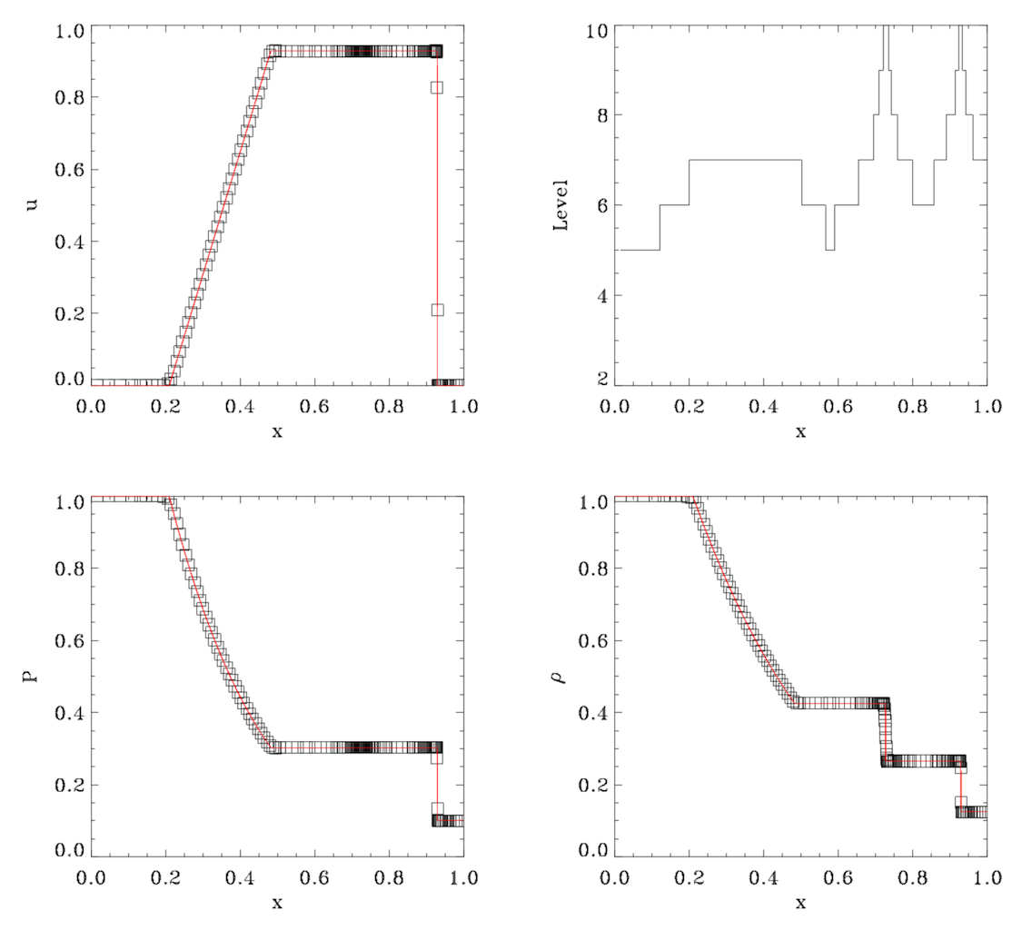
You can cut and paste the 142 lines into another file and use your
favorite data viewer like xmgrace or gnuplot to visualize the
results. These should be compared to the plots shown on the figure below. If
you have obtained comparable numerical values and levels of
refinements, your installation is likely to be valid. You are
encouraged to edit the parameter file tube1d.nml and play around
with other parameter values, in order to test the code
performances. You can also use other parameter files in the
namelist/ directory
If you would like to run a 2D simulation (using file sedov2d.nml for
example), do not forget to recompile entirely the code using:
$ cd trunk/ramses/bin
$ make clean
$ make NDIM=2
This last image shows the numerical results obtained with ramses for the Sod shock tube test (symbols) compared to the analytical solution (red line).