Mesh data structures #

Several data structures are used to keep track of the cells in the grid. We go into the purpose of each of them.

1. Octree representation of the computational domain #

To represent the grid, RAMSES uses an octree structure which can be refined locally. The computational domain is divided into grids (classically called octs): collections of 2$^\texttt{ndim}$ cells (8 in 3D) where ndim is the number of dimensions. On level 1, we start with 1 grid containing 2, 4 or 8 cells which span the entire computational domain. The maximum number of cells in each dimension for a refinement level $L$ is 2$^L$.

Remarkt that the number of cells in a grid is a quantity that is often used in the code, and so it has its own decided variable: 2$^\texttt{ndim}=$twondim.

To keep track of the relation between cells and grids of different refinement levels, ramses stores three arrays. They defined in the module amr_commons and allocated in the subroutine init_amr:

integer ,allocatable,dimension(:)  ::son     ! son grid
integer ,allocatable,dimension(:)  ::father  ! father cell
integer ,allocatable,dimension(:,:)::nbor    ! neighboring father cells

allocate(son   (1:ncell))
allocate(father(1:ngridmax))
allocate(nbor  (1:ngridmax,1:twondim))

A schematic example for two refinement levels in a 2D grid:

$image1$ $image2$

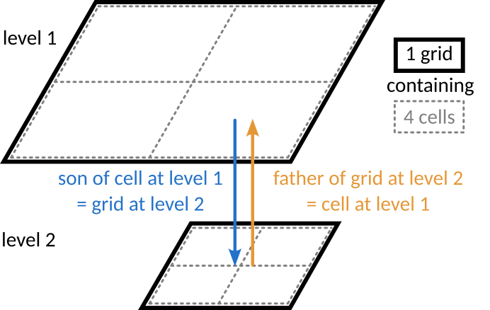
If a cell is refined, the array son contains the index of the child grid of the cell, from which the 2$^\texttt{ndim}$ children cells can be accessed. If the cell is not refined, its son is set to 0.
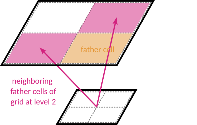
A grid at level L has a parent cell at level L-1. The array father stores for each grid the index of their parent cell.
The father cell of a grid has two directly neighoring cells in each spatial direction (2 in 1D, 4 in 2D and 6 in 3D). The refinement rules dictate that these neighbors exist on the level (but they may be refined themselved). The indices of these neighbors are stored in the array nbor, which is a 2D array of size [ngridmax, 2 x ndim].

Exercise

Using the arrays defined above, how can you get the $2 \times \texttt{ndim}$ directly neighboring grids of a grid at index igrid?

Solution

do j=1,twondim
   neighbor_grid(j) = son(nbor(igrid, j))
end do

This is implemented in the routine getnborgrids in amr/nbors_utils.f90.

2. Grid versus cell based arrays #

In general, AMR grid related arrays are defined in amr_commons.f90, and allocated in init_amr.f90. Arrays can be either grid-based or cell-based, which determines their size at allocation:

allocate(grid_based_array(1:ngridmax))
allocate(cell_based_array(1:ncell))

When running a simulation, the user specifies the number of grids to be allocating for working memory through the parameter ngridmax. Remark that this is the number of grids or cells allocated for each MPI process. Alternatively, the user can specify the total number of grids over the entire simulation domain using ngridtot=ngridmax*ncpu. This is then converted to ngridmax to be used in the remainder of the source code. Do not use ngridtot inside your code, other than to convert to ngridmax.

The corresponding number of cells is then ngridmax multiplied by 2$^\texttt{ndim}$, plus the number of cells at the coarses level that takes to take into account the physical bounderies:

ncell=ncoarse+twotondim*ngridmax

The cells inside a grid are stored in a specific order. Their position is typically indicated by the variable ind which goes from 1 to 2$^\text{ndim}$ (twotondim). In a cell-based array, all cells with ind=1 are stored first, followed by all those with ind=2, etc. A schematic example in 2D:

$image3$

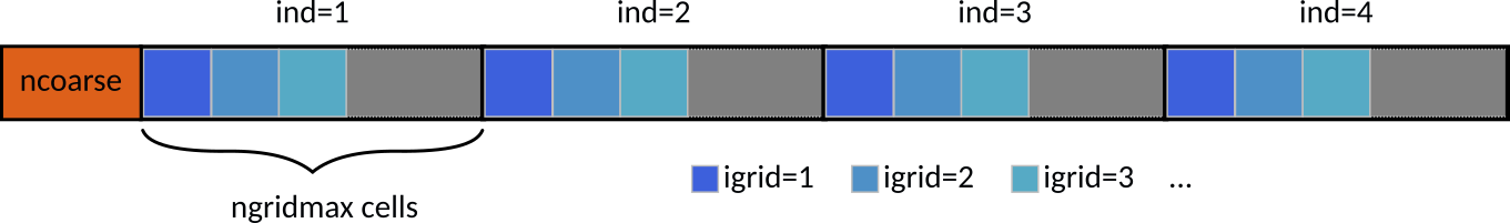
Added at the beginning of the list is the root cell and the coarse cells for the physical boundaries, a total of ncoarse cells, with ncoarse=nx*ny*nz. In the case of periodic boundary conditions nx=ny=nz=1, meaning the only coarse cell is the root cell of the octree at level 0.

How exactly the positions ind are defined in space is a matter of arbitrary convention. Variables that define the spatial relations between neighboring grids and cells can be found in amr_constants, for example lll and mmm, and in the routines in amr/nbors_utils.f90. They are used, for example, in the neighbor-searching routines (see further). simply want to access all neighbors, and the spatial order is irrelevant.

Exercise

Given the index of a cell icell, how can we obtain the index of the grid to which it belongs?

Solution

! Get the cell's position in its grid, that is the
! index ind, between 1 and twotondim.
ind=(icell-ncoarse-1)/ngridmax+1  !integer devision

! Convert the cell's index to the index of its grid
iskip=ncoarse+(ind-1)*ngridmax
igrid=icell-iskip

3. Linked list variables #

The grids making up the computational domain are stored in a linked list using an ordering recipe chosen by the user. For more on ordering, see the chapter on Domain decomposition.

A linked list is a chain of individual elements where each element knows about the next (index array next) and the previous element (index array prev) in the list. In RAMSES, these variables are defined in the module amr_commons and allocated in the subroutine init_amr:

integer ,allocatable,dimension(:)  ::next    ! next grid in list
integer ,allocatable,dimension(:)  ::prev    ! previous grid in list

allocate(next  (1:ngridmax))
allocate(prev  (1:ngridmax))

This makes it easy to insert new elements at any location, when a grid is created as a result of AMR refinement. Grids can also easily be removed when de-refinement occurs. A grid can be removed by connecting its previous element to the next element. Remark that these are grid-based arrays.

A linked list is stored for each MPI process (cpu) and AMR level. RAMSES keeps track of

headl: the index of the head, i.e. the first element in the list
taill: the index of the tail, i.e the last element in the list
numbl: the number of elements in the list

! Pointers for each level linked list
integer,allocatable,dimension(:,:)::headl ! Head grid in the level
integer,allocatable,dimension(:,:)::taill ! Tail grid in the level
integer,allocatable,dimension(:,:)::numbl ! Number of grids in the level

! Allocate linked list for each level
allocate(headl(1:ncpu,1:nlevelmax))
allocate(taill(1:ncpu,1:nlevelmax))
allocate(numbl(1:ncpu,1:nlevelmax))

At the start of the simulation, ngridmax grids are allocated. As mentioned before, this parameter needs to be set in the namelist. These ngridmax grids are divided amongst the following three linked lists:

headl, taill and numbl: the main computational domain inside an mpi process
headb, tailb, numbb: physical boundary grids around the computational domain
headf,tailf,numbf: unused grids (free memory)

A grid can only be part of one list at a time.

Exercise:

Given how the linked list is stored, write some code to remove a grid igrid from the linked list of refinement level ilevel in the MPI domain icpu. Think about all the possible positions in the linked list the grid could be.

Solution

if(prev(igrid).ne.0) then
   if(next(igrid).ne.0)then
      ! grid is somewhere in the middle of the list
      next(prev(igrid))=next(igrid)
      prev(next(igrid))=prev(igrid)
   else
      ! grid is at the tail of the list
      next(prev(igrid))=0
      taill(icpu,ilevel)=prev(igrid)
   end if
else
   if(next(igrid).ne.0)then
      ! grid is at the head of the list
      prev(next(igrid))=0
      headl(icpu,ilevel)=next(igrid)
   else
      ! grid is the only item in the list
      headl(icpu,ilevel)=0
      taill(icpu,ilevel)=0
   end if
end if
numbl(icpu,ilevel)=numbl(icpu,ilevel)-1

The code for removing grids from the linked list can be found in the subroutine kill_grid, in the file amr/refine_utils.f90. In this routine, a specified number of grids are removed and their corresponding variables reset to zero. We go into this further in the section on refinement.

Exercise

Analogously to the previous exercise, write code to add a grid igrid to the end of the linked list of refinement level ilevel in the MPI domain icpu.

Solution

if(numbl(icpu,ilevel)>0)then
   next(igrid)=0
   prev(igrid)=taill(icpu,ilevel)
   next(taill(icpu,ilevel))=igrid
   taill(icpu,ilevel)=igrid
   numbl(icpu,ilevel)=numbl(icpu,ilevel)+1
else
   next(igrid)=0
   prev(igrid)=0
   headl(icpu,ilevel)=igrid
   taill(icpu,ilevel)=igrid
   numbl(icpu,ilevel)=1
end if

The subroutine make_grid_fine in the file amr/refine_utils.f90 handles adding new grids. This routine does various things (see section refinement). The part that updates the linked list can be found under the comment !Connect news grids to level ilevel linked list. Remark that a seperate routine exists for adding cells at level 1: make_grid_coarse. The last code block of this routine handles the linked list update.

4. The variables `active` and `boundary`#

One way to access the grids for processing them, is to simply iterate throught the linked list by starting at the headl and following next. This is however not always practical. Instead, the grid indices are gathered in advance, by iterating through the linked lists and storing them in the variable active. An equivalant exists for the grids in the physical boundary, named boundary. These variables are defined in amr_commons:

type(communicator),allocatable,dimension(:)  ::active    ! 1:nlevelmax
type(communicator),allocatable,dimension(:,:)::boundary  ! 1:MAXBOUND,1:nlevelmax

They are arrays of a costume defined data structure called communicator. Derived types in fortran are analogous to structs in C/C++. To access its members, the synthax % is used. A communicator has various fields, but for keeping track of the grids only two are used:

type communicator
  integer                            ::ngrid   ! number of grids
  integer     ,dimension(:)  ,pointer::igrid   ! list of grid indices
  ...
end type communicator

(More on communicators in the Chapter on MPI communication). This data structure contain a list of the index of each grid, as found by iterating over the linked grid list (head, next).

The array active holds a communicator for each AMR level of the current MPI domain with ID myid. Each communicator the contain a list of the index of each grid, as found by iterating over the linked grid list usingheadl and next. The array boundary is similar, but instead keeps track of the different physical boundary regions for each level. Its contents is gathered by starting at headb.

Exercise

Write code to fill active(ilevel) of the current MPI domain by iterating through the corresponding linked list.

Solution

ncache=numbl(myid,ilevel)
! Reset old communicator
if(active(ilevel)%ngrid>0)then
   active(ilevel)%ngrid=0
   deallocate(active(ilevel)%igrid)
end if
if(ncache>0)then
   ! Allocate grid index to new communicator
   active(ilevel)%ngrid=ncache
   allocate(active(ilevel)%igrid(1:ncache))
   ! Gather all grids
   igrid=headl(myid,ilevel)
   do jgrid=1,numbl(myid,ilevel)
      active(ilevel)%igrid(jgrid)=igrid
      igrid=next(igrid)
   end do
end if

The arrays active and boundary are synchronised with the linked list in the subroutine build_comm in virtual_boundaries.f90, which builds the communication structure for a specified AMR level.

5. Processing grids and cells #

Iterating through grids #

To process grids, we can now simply use active which contains the grids that are actually in use. To iterate through the grids, use the following straighforward code pattern:

do i=1,active(ilevel)%ngrid
   some_grid_array(active(ilevel)%igrid(i))=something
end do

Iterating through cells #

Most of the arrays we want to process are however cell-based instead of grid-based. Remember that for each grid, there are 2$^\mathrm{ndim}$ cells stored according to the pattern:

$image3$

A variable iskip gives the number of elements to skip when looping over the grids and processing all cells at position ind:

iskip=ncoarse+(ind-1)*ngridmax

A commonly found loop pattern in the code is then:

do ind=1,twotondim
   iskip=ncoarse+(ind-1)*ngridmax
   do i=1,active(ilevel)%ngrid
      some_cell_array(active(ilevel)%igrid(i)+iskip)=something
   end do
end do

where the outer loop goes over the position of the cells inside the grids, while the inner loops go over the grids. When accessing multiple arrays, the cell indices are typically calculated in advance (for the current vector sweep, see next section). An example:

do ind=1,twotondim
  ! gather cell indices
  iskip=ncoarse+(ind-1)*ngridmax
  do i=1,ngrid
    ind_cell(i)=iskip+ind_grid(i)
  end do
  ! Compute pressure from temperature and density
  do i=1,ngrid
    uold(ind_cell(i),neul)=uold(ind_cell(i),1)*uold(ind_cell(i),neul)
  end do
end do

Nvector sweeps #

Nowadays, CPUs are able to operate on multiple values at once that are located in neighboring memory locations. This only works if the exact same operation is to be executed, that is without if-else branching. The memory layout of the AMR-tree can however be complex, possibly leading to unfavorable memory access-patterns. To circumvent this problem, explicit vectorization using the compile-time parameter NVECTOR is build-in in RAMSES.

An standard loop structure in RAMSES then looks like this:

! Loop over active grids by vector sweeps
ncache=active(ilevel)%ngrid
do igrid=1,ncache,nvector
   ngrid=MIN(nvector,ncache-igrid+1)
   do i=1,ngrid
      ind_grid(i)=active(ilevel)%igrid(igrid+i-1)
   end do
   call calculation_routine1(ind_grid,ngrid,ilevel)
end do

This is going to gather the indices of nvector grids before sending them off to a calculation routine. An example can be found for the hydro solver, where in the routine godunov_fine grids are send to the routine godfine1, which is the entry point for the actual calculation.

The size of nvector has a strong impact on code performance. A large nvector may lead to a better vectorization rate, but small nvector values are better for hardware cache performance. The best value is dependent in the machine and the type of simulation.

6. Finding neighbors #

Routines to find neighboring cells and grids are implemented in the file amr/nbor_utils.f90. While in most cases, we can simply make use of these routines, it is insightfull to understand how they work. As an exercise, we will go through the process of finding neighbors in 1D, where two configurations are possible:

$image4$

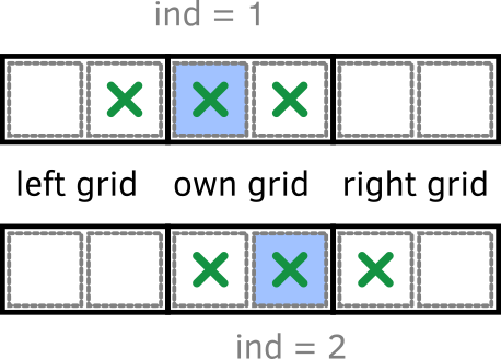
Exercise (part 1):

In the case of 1D, what are the steps to find the neighboring cells of a given cell? We want the center cell to be included in the list of neighbors. The input of the routine will be the index of the cell.

Solution

Step 1: Determine the position of the cell in its grid.
Step 2: Determine the index of the grid to which the cell belongs.
Step 3: Get the neighboring grids of the grid found in step 2.
Step 4: Using the position found in step 1, determine which of the grids found in step 3 actually contain the neighbor cells.
Step 5: Using the position found in step 1, find for each neighbor cell the position in its grid (the grids found in step 4)

Exercise (part 2):

Write (pseudo-)code to execute each of the steps found in part 1 of the exercise.

Exercise (part 3):

Take a look at the different routines that are implemented in the file nbor_utils.f90. Which routine serves which purpose? Which routine could be used to get the neighboring cells in 1D? Compare your (pseudo-)code to what is implemented in nbor_utils.f90

Solution

The 1D case is a bit of a special case, because there is no distinction between getting the direct neighbors or also including diagonal neighbors (since there are no diagonals…). You could either use the implementation the routine getnborgrids or get3cubefather.

Exercise (part 4):

What would change in the case of 2D? Make a distinction between retrieving the 4 direct neighbors and including also the diagonal neighbors.

Mesh data structures

Contents