MPI communications#
Domain decomposition over MPI processes#
Hilbert curve#
Several recipes exist to divide the cells making up the computational box into individual domains to be assigned to MPI processes. The default, and most commonly used in RAMSES, is Hilbert domain decomposition. The decomposition curve will assign to each location in a multi-dimensional space a one-dimensional order. By setting the namelist parameter ordering in the RUN_PARAMS block, users could choose options other than Hilbert.
An example of the Hilbert curve in a 2D computational domain and the resulting domain decomposition is shown below:
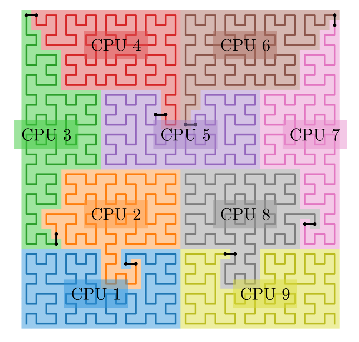
Credits: Cadiou (2019).#
The index indicating a cell’s position in the 1D Hilbert curve (or any other ordering recipe) is stored in the global array hilbert_key, defined in amr_commons
real(qdp),allocatable,dimension(:)::hilbert_key
and allocated in init_amr:
allocate(hilbert_key(1:ncell)) ! Ordering key
hilbert_key=0.0d0
Note that the Hilbert curve is always defined on levelmax. This means that when using deep levels of refinement (levelmax >19), the value of the index on the curve may be so large that it does not fit into a regular double precision real number. In this case, one should compile with QUADHILBERT, which increases the size of the elements of the array hilbert_key:
#ifdef QUADHILBERT
  integer,parameter::qdp=kind(1.0_16) ! real*16
#else
  integer,parameter::qdp=kind(1.0_8) ! real*8
#endif
CPU map#
To distribute the cells over the MPI domains, the Hilbert curve is then cut into “equal” part according to some recipe (see further).
The variables keeping track of which cell is in which MPI domain are defined in amr_commons and allocated in init_amr
integer ,allocatable,dimension(:)  ::cpu_map  ! domain decomposition
integer ,allocatable,dimension(:)  ::cpu_map2 ! new domain decomposition
! Allocate MPI cell-based arrays
allocate(cpu_map    (1:ncell)) ! Cpu map
allocate(cpu_map2   (1:ncell)) ! New cpu map for load balance
cpu_map=0; cpu_map2=0
They are used in the load balancing.
Load balancing#
Load balancing is the operation of redistributing the computational load between the MPI domains. The main routine load_balance can be found in the file amr/load_balance.f90. It goes through the following steps. * Compute new cpu map using the chosen ordering (usually Hilbert) * Expand boundaries to account for new mesh partition * Update physical boundary conditions * Rearrange octs between cpus * Compute new grid number statistics * Set old cpu map to new cpu map * Shrink boundaries around new mesh partition
The computational cost is estimated with a simple heuristic, assuming (by default) the cost to be level-dependent
where \(f_\ell = \prod_{\ell'=\ell_\mathrm{min}}^{l} N_{\mathrm{subcycle},\ell'}\) is the product of the number of subcycles compared to the base grid (related to adaptive time stepping). \(a\) and \(b\) are magic numbers. By default, \(a=80\) and \(b=1\) (i.e., an oct costs 80 more than a particle).
Ghost zones#
Example of ghost zones: the light-shaded cells are “known” by both CPU1 and CPU2 in this example, and represent shared ghost zones.
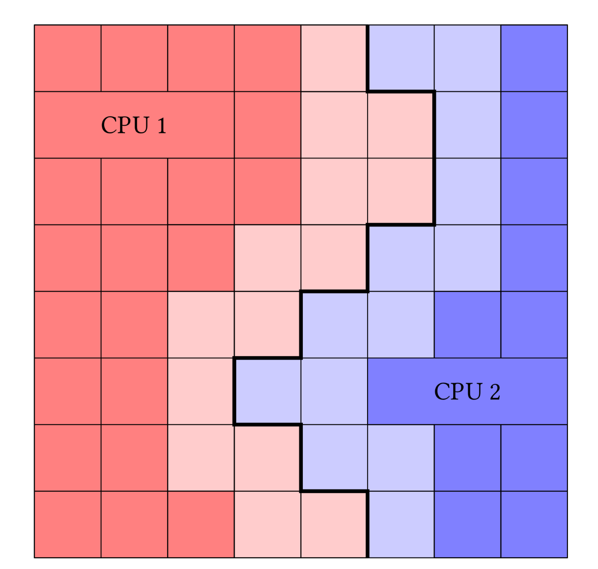
Credits: Cadiou (2019).#
The ghost zones are replicated on the relevant processors to construct locally essential trees, such that each local octree contains all the necessary information for the computations (until communications are needed). The figure below shows an example of ghost zones and corresponding tree stored on different MPI process (from Romain Teyssier lecture):
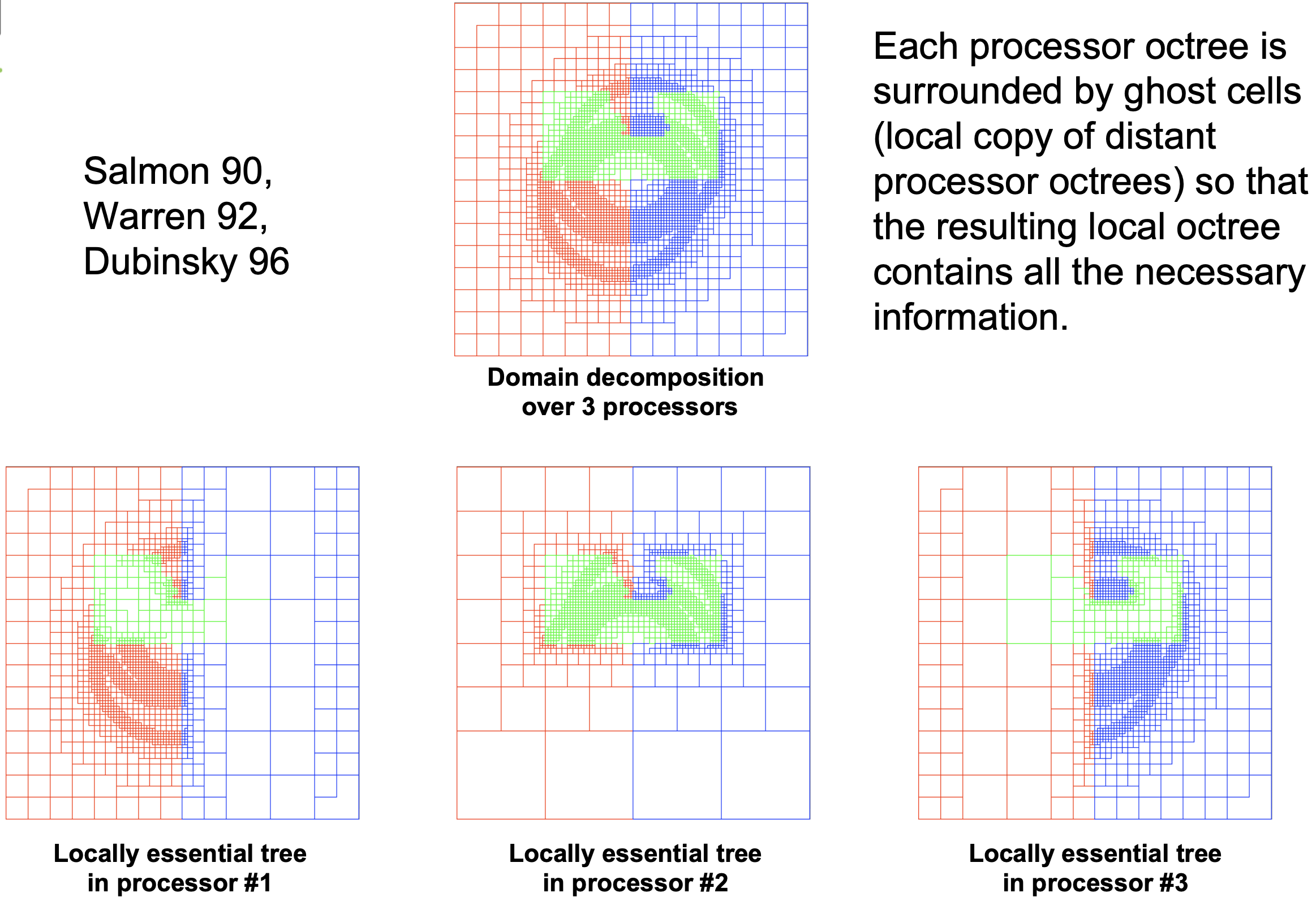
Credits: Romain Teyssier’s lectures.#
Communication between MPI domains#
Communicator variables#
RAMSES defines the derived type communicator. Derived types in fortran are analogous to structs in C/C++. To access its members, use %.
! Communication structure
type communicator
  integer                            ::ngrid   ! number of grids
  integer                            ::npart   ! number of particles
  integer     ,dimension(:)  ,pointer::igrid   ! list of grid indices
  integer     ,dimension(:,:),pointer::f       !
  real(kind=8),dimension(:,:),pointer::u       !
  integer(i8b),dimension(:,:),pointer::fp      !
  real(kind=8),dimension(:,:),pointer::up      !
end type communicator
In classic RAMSES, four global communicator arrays are defined in amr_commons:
! Active grid, emission and reception communicators
type(communicator),allocatable,dimension(:)  ::active     ! 1:nlevelmax
type(communicator),allocatable,dimension(:,:)::boundary   ! 1:MAXBOUND,1:nlevelmax
type(communicator),allocatable,dimension(:,:)::emission   ! 1:ncpu,1:nlevelmax
type(communicator),allocatable,dimension(:,:)::reception  ! 1:ncpu,1:nlevelmax
Remark that active and boundary are not for communication, they are simply used to easy book-keeping of the grids. Only the fields ngrid and igrid are used for these (see the chapter on grid data structures).
The arrays emission and reception are for actual MPI communication. These arrays are altered by the light MPI implementation to have a smaller memory imprint. They are used both for ghostzone and particle communication.
Ghost zone communication#
To communicate the values of the different global arrays in the ghost zones, RAMSES uses the routines in amr/virtual_boundaries.f90.
make_virtual_fine(forward exchange) Fill the ghost zones (virtual grids) of neighboring MPI domains with up-to-date values from inside current MPI domain. Steps:launch asynchronous receives from the other CPUs (send to
receptioncommunicator)gather the local data that is to be send to the neighboring domains into the
emissioncommunicatorlaunch asynchronous sends to the other CPUs
wait for all receives to complete
copy the received data from the reception buffer to the correct index in the global array
wait for sends to complete
make_virtual_reverse(reverse exchange) Send data from the current MPI domain’s virtual grids to real grids of neighboring domains. Contributions are added to the field:xx(igrid) = xx(igrid) + received_value. This needs to be done after an update that affect neighboring cells has been performed, i.e., the computation of hydro fluxes and computation of the density field using CIC. For the coarsest levels, sychronous SEND/RECV are used. For the finer levels, a simimal asynchronous send/recv pattern is uses as in the forward exchange.
There are two versions of the make_virtual_fine and make_virtual_reverse subroutines: one for communicating floating point numbers (_dp) and one for integers (_int). They are nearly identical. The only differences are:
the field accessed in the emission/reception communicators (
ufor doubles,ffor integers),the MPI types in the SEND/RECV calls (MPI_DOUBLE_PRECISION and MPI_INTEGER respectively).
Exercise
For hydro, which array should be used uold and unew? It depends on the exchange(reverse versus forward).
Solution
It is linked to set_unew
Particle communication#
Particles move freely in the computation domain, which means they can travel to other MPI domains. This is handeled by virtual_tree_fine in pm/particle_tree.f90.
When to communicate?#
Communications must be done each time a global array, e.g., uold, is modified (i.e., after cooling or feedback), to inform the neighbor process about the change, using make _virtual_fine.
Exercise
Find other arrays that are communicated. Why is make _virtual_reverse called only for unew, phi and rho?
Solution
make_virtual_reverse in only needed when a flux in applied at a MPI domain boundary, or when a particle belonging to on MPI process deposit mass on a neighboring MPI domain. phi is used as temporary array in rho_fine.f90.