Refinement schemes & implementation#
Please make sure to read the lecture on the AMR structure before following this lecture on the refinement criterions
1. What is refinement about?#
1.1 Introduction#
Refinement is the process of adapting the grid to the physical state of the simulation, by increasing or decreasing the resolution according to user-refinement criteria. In RAMSES, which uses a cell-based adaptive mesh, this consists in creating or destroying grids (i.e. a set of \(2^{\mathrm{ndim}}\) cells) when needed. Contrary to other codes, RAMSES does not have a derefinement criteria: a refined grid is marked for derefinement as soon as it no longer satisfies the criterion for refinement. In addition to the user-defined criteria, RAMSES ensures that the refinement map follows some geometrical rules that simplify the implementation of the Godunov solver and help with the stability of the numerical scheme.
1.2 General description#
Let first review the description of the refinement algorithm in Teyssier 2002.
Click to read
The first step consists of marking cells for
refinement according to user-defined refinement criteria, within
the constraint given by a strict refinement rule: any oct in the
tree structure has to be surrounded by \(3^{ndim} − 1\)
neighboring parent cells. Thanks to this rule, a smooth transition
in spatial resolution between levels is enforced, even in the
diagonal directions. Practically, this step consists in three
passes through each level, starting from the finer level
levelmax down to the coarse grid \(l = 0\).
| 1. If a split cell contains a children cell that is marked or
already refined, then mark it for refinement; 2. Mark the
\(3^{ndim} − 1\) neighboring cells 3. If any cell satisfies the
user-defined refinement criteria, then mark it for refinement.
One key ingredient still missing in this procedure is the so-called
“mesh smoothing”. Usually, refinement are activated when gradients
(or second derivatives) in the flow variables exceed a given
threshold. The resulting refinement map tends to be “noisy”,
especially in smooth part of the flow where gradients fluctuates
around the threshold. […] [To avoid this, in Ramses], a cubic buffer
is expanded several times around marked cells. The number of times
one applies the smoothing operator on the refinement map is obviously
a free parameter. This parameter is noted nexpand. […] Note that
the exact method implemented here […] leads to a convex structure for
the resulting mesh, that is likely to increase the overall stability
of the algorithm. Note also that only refinement criteria are
necessary in RAMSES: no de-refinement criteria need to be specified
by the user. Since the refinement map has been carefully built during
[this] step, the refinement rule should be satisfied by construction.
This is however not the case if one uses the adaptive time step
method […] . In this case, a final check is performed before
splitting leaf cells. If the refinement rule is about to be violated,
leaf cells are not refined.
The next step consists in splitting or destroying children cells according to the refinement map. RAMSES performs two passes through each level, starting from the coarse grid up to the finer grid 1. If a leaf cell is marked for refinement, then create its child oct; 2. If a split cell is not marked for refinement, then destroy its child oct.
Creating or destroying a child oct is a time-consuming step, since it implies reorganizing the tree structure. Thanks to the double linked list associated to the fully-threaded tree structure, this is done very efficiently by first disconnecting the child oct from the list, and then reconnecting the list in between the previous and next octs. Note however that this operation can not be vectorized. It is important to stress that this operation is applied at each time step, but for a very small number of octs. In other word, at each time step, the mesh structure is not rebuilt from scratch, but it is slightly modified, in order to follow the evolution of the flow.
In short, the refinement proceeds in two phases:
First go through all levels, starting from the finest, and marking (or flagging) cells that need to be refined according to the user-defined criteria. Doing so, the algorithm makes sures that the following rules are respected:
The 2:1 rule: If your neighbor is at level \(l\), your level should be \(l\) or \(l\pm1\). This ensures that at any boundary of a cell, you have either one neighbor (of level \(l\) or \(l - 1\)) or two (of level \(l + 1\)).
The smoothing rule: Every “physically” refined cell should be surrounded by at least
nexpandrefined cells in every directions.“Not too fast” derefinement rule: At each step, in any position, the refinement can only be reduced by one level
Split or merge the cells, according to the map built in first phase.
2. Flagging cells for refinement#
Building the refinement map is done by the routine flag in
amr/flag_utils.f90. It consists in filling the array flag1, with
information on which cells should be refined. The actual refinement (if
needed), is done in the next phase by the routine refine (see
Section TBD).
The array flag1 is defined in amr/amr_commons.f90 by
integer ,allocatable,dimension(:) ::flag1 ! flag for refine
and allocated in amr/init_amr.f90 by
! Allocate AMR cell-based arrays
allocate(flag1(0:ncell)) ! Note: starting from 0
where ncell is the maximal number of cells for one MPI process. It
is a cell-based array, meaning that flag1(icell) contains the flag
information for the cell icell of the current process. If
flag1(icell) == 1 it means that the cells should be refined at
during this time step, while flag1(icell) == 0 means it should not
be in a refined state (so derefined if it is currently refined).
In Ramses jargon, to flag or to flag1 a cell icell means
setting flag1(icell) to 1.
Warning
The array flag1 is also used in other part of the code
for various purposes (including load balance). The refinement
information is thus only stored and valid in the routinerefine,
which should be called just after flag.
The routine flag calls the routine flag_fine over each level,
starting from the finest one, and then the routine flag_coarse on
the coarse grid (i.e. \(l = 0\)). For each level, flag_fine
proceeds in 5 steps:
Show code
subroutine flag_fine(ilevel,icount)
use amr_commons
implicit none
integer::ilevel,icount
!--------------------------------------------------------
! This routine builds the refinement map at level ilevel.
!--------------------------------------------------------
integer::iexpand

if(ilevel==nlevelmax)return
if(numbtot(1,ilevel)==0)return

! Step 1: initialize refinement map to minimal refinement rules
call init_flag(ilevel)

! If ilevel < levelmin, exit routine
if(ilevel<levelmin)return
if(balance)return

! Step 2: make one cubic buffer around flagged cells,
! in order to enforce numerical rule.
call smooth_fine(ilevel)

! Step 3: if cell satisfies user-defined physical citeria,
! then flag cell for refinement.
call userflag_fine(ilevel)

! Step 4: make nexpand cubic buffers around flagged cells.
do iexpand=1,nexpand(ilevel)
   call smooth_fine(ilevel)
end do

! In case of adaptive time step ONLY, check for refinement rules.
if(ilevel>levelmin)then
   if(icount<nsubcycle(ilevel-1))then
      call ensure_ref_rules(ilevel)
   end if
end if

end subroutine flag_fine
Step 1: Initialisation#
The subroutine init_flag(ilevel) builds the initial state at each
level. It first initializes the flag1 array at zero, as this array
has been altered in other part of the code for other purposes. Please
pay attention on how we go through all the active cells of a given level
since this is used quite a bit here.
! Initialize flag1 to 0
nflag=0
do ind=1,twotondim
   iskip=ncoarse+(ind-1)*ngridmax
   do i=1,active(ilevel)%ngrid
      flag1(active(ilevel)%igrid(i)+iskip)=0
   end do
end do
Then, cells are flagged depending on the state of their childeren (if
they have any). This is done in the test_flag subroutine. If
son(icell)>0 the cell is currenlty refined. We then loop over the
children cells to see if any of them * a) has been already flagged for
refinement, i.e. has flag1(i_child_cell)=1, which is known because
the flagging operation is done level by level, starting from the finer
ones, * b) is currently refined.
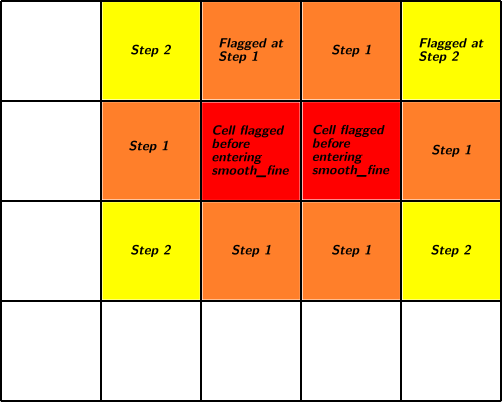
If any of these conditions is true, the cell is flagged. Three example situations are show in the figure below.
By flagging the cells that contain refined cells, we keep them in their refined state, ensuring the “Not too fast” derefinement rule is respected (see the middle example).
Of course, in levels below levelmin, all cells are marked for
refinement.
Step 2: Cubic buffer#
The next step consist in marking the \(3^\mathrm{ndim} − 1\)
neighboring cells of each one of the cells marked at step 1. This is
performed by the smooth_fine subroutine. This ensures that 2:1
rule is respected (as long as all the levels are flagged in this
timestep, ie no adaptive timestepping is used - see Step 5).
The smooth_fine routine proceeds in ndim iterations: - iteration
1: flag1 cells with at least 1 flag1 neighbors (if ndim > 0) -
iteration 2: flag1 cells with at least 2 flag1 neighbors (if ndim >
1) - iteration 3: flag1 cells with at least 2 flag1 neighbors (if
ndim > 2)
In each step, it uses the flag2 array as a temporary array, because
we want to distinguish the cells that were flagged before entering the
step from the ones flagged during the step. flag2 is built the same
way as flag1.
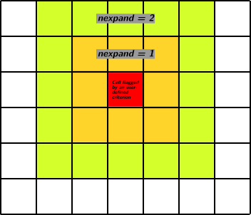
By doing so, it ensures that each previously flagged cells will be surrounded by flagged cells (see illustration below)
Step 3: Apply user-defined criterion#
This is where you may want to change things
Cells are flagged according to a user specified criterion in the routine
userflag_fine. The different criteria are detailled in the next
section.
In cosmo runs, the whole level is prevented to refine in certain conditions.
There are several subroutines for refinement criteria:
- subroutine
flag_utils.f90/poisson_refine(): local Lagrangian and variable
refinement criteria, based on the mass (or another variable) in each
cell, using the parameters m_refine, ivar_refine,
var_cut_refine:
- subroutine godunov_utils.f90/hydro_refine():
error on gradients (parameters err_grad_d, err_grad_p,
err_grad_u, rt_err_grad_xHII, rt_err_grad_xHI, as well as
MHD variables ) - subroutine
godunov_utils.f90/jeans_length_refine(): refinement over the jeans
length (parameter jeans_refine)
- subroutine rt_hydro_refine(): refinement over rt_err_grad_cn.
After each of these routine, a bunch of new cell are flagged as to be
refinable using the temporary array ok array. There is then an
additional filter implementing the geometrical refinement (subroutine
geometry_refine), that will unmark all the cells that do not
fulffill it by updating the ok array. By using a temporary array
instead of flag1, there is no risk of breaking the refinement rules)
[1]. Finally all the cells marked with
okare marked withflag1.
Step 4: Mesh smoothing#
Enforce the smoothing rule. This simply applies the smooth_fine()
subroutine, that was used in step 2, nexpand times.
Step 5: Ensure the 2:1 refinement rule (if we are in an adaptive step)#
Step 1-4 ensure that the refinement rules are always respected, as long as they are applied to all levels.
However, if adaptive timestepping is used, it may well be that the
flag_fine routine applied at level ilevel but not at level
ilevel - 1 [2], and thus that the planned refinement may break
the 2:1 rule. If we are within such a timestep, that is if icount
(the current subcycling step at this level) is not the last one
(nsubcycle(ilevel-1)), we call the ensure_ref_rules subroutine.
This subroutine goes through each grid \(i\) at level ilevel and
makes sure that all the \(2^\mathrm{ndim}\) neighboring grids
exists. If this is not the case, the cells within the grid i cannot
be refined without potentially breaking the 2:1 rule and are unflagged.
Warning
Note that because of this, the mesh smoothing rule with nexpand >
2 is actually not ensured.
3. Existing user defined criteria#
In this section, we review how the existing user-defined criteria are
implemented. They are controlled by the REFINE_PARAMS namelist block
(see the doc
here).
3.1. Mass (“Quasi Lagrangian strategy”)#
This corresponds to the parameters m_refine, mass_sph and
mass_cut_refine and is applied in the poisson_refine routine.
The idea is to compute the total mass in each cell (including the
contrinution for particles), and comparing it to a reference mass
mass_sph. If the computed mass exceed
m_refine(ilevel) * mass_sph, the cell is refined. The mimics the
typical refinement of SPH codes.
Danger
In this part of the code, the arrays cpu_map and phi are used
as temporary array to flag the cells that should be refined and the
total “Lagrangian” mass in each cell. This allows to save memory and
allocation time and works because the information that was stored in
these arrays is no longer needed in the flag routine.
The routine works differently depending on whether gravity is turned on or not.
If poisson == .true., prior entering the flag_fine routine, the
array cpu_map is filled with a pre-refinement map, containing 1 for
the cells that should be refined according to quasi lagragian strategy,
and 0 for the others. This is done in the rho_fine routine in
pm/rho_fine.f90 where the total density field for the gravity is
calculated (the mass-refine information comes almost for free there).
The routine rho_fine firsts initialize the phi array (strange
name again, because this is also a reused array) with the mass of gas in
each cell divided by mass_sph. The contribution of the particles is
then added using the cloud-in-cell scheme. The map is then computed
(stored in cpu_map) by comparing the array phi with
m_refine(ilevel). In poisson_refine, we just use the content of
the array cpu_map to set the array ok, which is then used to
update the array flag1.
If poisson == .false., the mass of the gas in the cell is simply
compared to m_refine(ilevel) * mass_sph.
3.2 Variables and passive scalar strategy#
The user can also refine the initial grid by inputing a threshold on
the value of a variable. This is controlled by the ivar_refine and
var_cut_refine parameters. Cells where the hydro variable with the
index ivar_refine has a value larger than var_cut_refine should
be refined.
Warning
This refinement strategy is only working when gravity is on
(poisson == .true.)
This is also carried on within the poisson_refine and the
rho_fine routines. It acts as a filter on the quasi-lagrangian
strateg by preventing the refinement on the mass whenever
uold(ivar_refine)/rho < var_cut_refine.
3.3. Gradients (hydro and rt) strategy#
This refines on the gradients of user defined variables. The logic is simpler (compute the gradients and then apply the criterion), but the routines are spread among several files.
Exercise
Follow the different calls of hydro_flag and then
rt_hydro_flag to see when the array ok is updated. Did you
notice something strange with rt_hydro_flag?
3.4. Jeans length strategy#
This strategy is used a lot in simulations that care about the Truelove criterion, which says that to avoid artifical fragmentation of the gas, its Jeans length should be resolved by at least 4 cells.
It is also applied in the hydro_flag routine, which calls
jeans_length_refine which is computing the Jeans length and applying
the criterion.
3.5. Geometrical strategy#
This is actually a filter on the other kinds of refinement, which is ran
after all the previous criteria filled the ok array. Only the cells
that have ok(icell) == 1 and satisfy the geometrical criterion are
actually flagged to be refined (in flag1). Namely, the user has to
define a zone at each level in which the refinement can happen.
Exercise 1: Refine on a variable or a combination of variables#
Level 1#
Modify the “Variables and passive scalar” strategy to make it more
useful:
1. Make the “Variables and passive scalar” strategy independent
from the “Quasi Lagrangian strategy” (you can code it as a new strategy,
with its own parameters).
2. Make it possible to have a different
threshold at each level (ie make var_cut_refine an array)
Level 2#
If you have time, you can also decide to refine on a combination of variables. You will read and parse a formula from the namelist and refine on the result.
Exercise 2: Improve the geometrical criterion#
Modify geometry_refine to add more than one region of refinement,
allowing for more complex shapes.
Clue 1
You can take inspiration from the initial condition
“regions” parameters, which allows up to MAXREGION regions to be
initialized with different parameters.
Clue 2
Helping TODO List:
☐ In
amr_parameters, add aMAX_REGION_REFINEparameter☐ Add a new parameter
refine_params/nregions_refine(look at the appropriate lecture to see how to do that)☐ Change how
r_refine,x_refine, etc .. (up tob_refine) are defined. They could look likereal(dp),dimension(1:MAXLEVEL,1:MAXREGION)Look at clue 3 to see how to deal with multidimensional arrays in the namelist. Ideally we want to make sure of not introducing any breaking changes.☐ Now the hard work is in
geometry_refine. You need to introduce the appropriate loops. Beware of the logic:geometry_refineis a filter: if we have two regions we want to refine cells that are in region 1 OR region 2 [3]. You may want to use theflag2array as a temporary array.☐ Test your new implementation! First run the test suite to make sure you didn’t break anything, and then add a test that uses your improved geometrical criterion.
Clue 3
Deal with multidimensional arrays in the namelist: there’s some help in StackOverflow You can play with the following program (eg. with Online Fortran Compiler)
program test

   implicit none

   integer :: ierr, unit, i, ilevel, iregion
   integer,parameter :: MAX_REGION  = 4
   integer, parameter :: MAX_LEVEL = 3
   real(kind=kind(0.0d0)), allocatable :: p(:, :)

   namelist /VAR_p/ p


   allocate(p(MAX_LEVEL,MAX_REGION))
   open(newunit=unit, file='namelist.nml', status='old', iostat=ierr)
   read(unit, nml=VAR_p, iostat=ierr)
   close(unit)

   write(*,*) "REGIONS"

   do  iregion = 1,MAX_REGION
      write(*,*) p(:,iregion)
   end do

   write(*,*) "LEVELS"

   do ilevel = 1,MAX_LEVEL
      write(*,*) p(ilevel,:)
   end do
end program test
&VAR_p
!p = 1.30, 0.8, 3.1 ! Only one region, backwards compatible syntax
p(:,1) = 1.30, 0.8, 3.1 ! Region 1
p(:,2) = 1.50, 3.2 ! Region 2
/
4. Modify the tree structure#
In the previous step, we built a refinement map, stored in flag1,
whether each cell should be refined or not. Now it’s time to actually
apply the change, which consist adding a son grid in the leaf cells that
were marked for refinement (ie, splitting them) and were not refined
before, or destroy the son grid in refined cells that are no longer
flagged.
The is done is by the refine routine in amr/refine.f90. This
routine applies the refinement map on all levels, but this time going
from the coarsest level to the finest. The creation and destruction of
grid was discussed in the lecture on the mesh
structure.
An important question that arises when creating a cell is how to
interpolate the value of the variables. For the hydro variable, this is
done automatically by the code and controlled by the user with the
interpol_var and interpol_type parameters.
Warning
If you add a new variable, you may have to tell the code how to
interpolate it in the refine_utils/make_new_grid routine.